Friday, October 30, 2015

5 Tips for better DataStage Design


01.  Always try to complete the requirement first, Don't spoil your time to develop an optimized job which is practically useless until requirement is completed.

02.  To re-arrange an existing job design, or insert new stage types into an existing job flow, first disconnect the links from the stage to be changed, then the links will retain any meta-data associated with them.

https://blogger.googleusercontent.com/img/b/R29vZ2xl/AVvXsEh2iYZ7Pd_XtOhSaOpzef43FY6FF8xNua-hiaarGFi8jrAynO0TAjb4M5-ZXy_rq0pyq0CKZHcf-88oFiM7Otwda4xhN456mienXkRQzkP596Kx5CS6UEkCjWm5wEcPoHosEeXXG6jKnwk/s320/wordle+12.png


03.  A Lookup stage can only have one input stream, one output stream, and, optionally, one reject stream. Depending on the type of lookup, it can have several reference links. To change the use of particular Lookup   links in an existing job flow, disconnect the links from the Lookup stage and then right-click to change the link type, for example, Stream to Reference.

04.  The Copy stage is a good place-holder between stages if you anticipate that new stages or logic will be needed in the future without damaging existing properties and derivations. When inserting a new stage, simply drag the input and output links from the Copy place-holder to the new stage. Unless the Force property is set in the Copy stage, InfoSphere DataStage optimizes the actual copy out at runtime.

05.  DataStage takes longer to start-up a job for reasons such as it validates the entire environment, nodes and database connectivity before starting the ETL job. By doing so you have overheads upfront by it ensures robust and reliable data loading and integration. Parallel jobs are not recommended for small volume of data and serial fashion of ETL design, as there is an overhead is starting PX processes.

Thursday, October 29, 2015

Difference between Datastage 7.5X2,Datastage 8.0.1 and Datastage 8.5 Versions

Different Versions

DATASTAGE 8.5 ENHANCEMENTS

Datastage 8.5 Enhacements


It was  more faster than  before versiobs.
All the  tasks become faster than previous version 8.1 .

Tasks are like save, renaming, compiling etc.

The run time of the jobs has been improved.

In Datastage transformer Stage is one of the important stage.

In Datastage 8.5 , just got better than before version..

Transformer looping has been included in the transformer stage by I.B.M

There are two types of looping  available here.

Where we can output multiple O/P( Output )  links for single I/P( Input Link) Link.

For Example:

Input:

Marketing_person    City-1         city-2       city-3

James Bond         Washington     Newyork      Newjersey


Output will be

Marketing_person     City

James Bond         Washington
James Bond          New York
James Bond           New Jersey


This achieved  with the new system  variable @ ITERATION


System Variables:

@ ITERATION : used in the looping mechanism

LastRow(): Indicated the last row in the job

LastRowInGroup(): will return the last rown in the group based  on the key.

WHAT ARE THE CLIENT COMPONENTS IN DATASTAGE 7.5X2 VERSION
In Datastage 7.5X2 Version, they are 4 client Components. They are

1) Datastage Designer
2) Datastage Director
3) Datastage Manager
4) Datastage Admin

In Datastage Designer, We 

Create the Jobs
Compile the Jobs
Run the Jobs

In Director, We can 
View the Jobs
View the Logs
Batch Jobs
Unlock Jobs
Scheduling Jobs
Monitor the JOBS
Message Handling


In Manager , We can 
Import & Export the Jobs
Node Configuration

And by using Admin , We can 
Create the Projects
Organize the Projects
Delete the Projects


DataStage 8.1 to DataStage 8.5
1. DataStage Designer performance improvement By changing the Metadata algorythm, copy/delete/save jobs got faster about 30-40%.
2. Parallel Engine Performance and Resource improvements Resource usage is about 5% smaller than 8.1, for T-Sort, Windows desktop heap size has been decreased 94%.
3. Transformer enhancements Key break support
LastRowInGroup() function is added. This will return true for the last record of the group.
LastRow() will return the last record of input.
Output looping :: Allows multiple output records to be created per single input record.
Input looping    :: Allows aggregation of input records so that aggregated data can be included with the original input data. ( like adding average column to the original input is now possible. ( 2 pass.... calculation. )
New Null handling This is pretty complicate and need more verification by myself to explain clearly. But this is the description I got.
Null values can now be included in any expression.
        -> Null values no longer need to be explicitly handled.
            A null value in an expression will return a null value result. As long as the target column is nullable, records will not be dropped. Stage variables are now always nullable.

APT_TRANSFORM_COMPILE_OLD_NULL_HANDLING is prepared to support backward compatibility.

New Transformer Functions
Create/offset a time, date or timestamp from component arguments
DateFromComponents(int32 years, int32 months, int32 dayofmonth)
DateOffsetByComponents(date basedate, int32 yearoffset, int32 monthoffset, int32 dayoffset) DateOffsetByDays(date basedate, int32 offset)
TimeFromComponents(int32 hours, int32 minutes, int32 seconds, int32 microseconds) TimeOffsetByComponents(time basetime, int32 houroffset, int32 minuteoffset, dfloat secondoffset) TimeOffsetBySeconds(time basetime, dfloat secondoffset)
TimestampOffsetByComponents(timestamp basetimestamp, int32 yearoffset, int32 monthoffset, int32 dayoffset, int32 houroffset, int32 minuteoffset, dfloat secondoffset)
TimestampOffsetBySeconds(timestamp basetimestamp, dfloat secondoffset)

Various packed decimal conversions
DecimalToDate(decimal basedecimal [,string format] )
DecimalToTime(decimal basedecimal [,string format] )
DecimalToTimestamp(decimal basedecimal [,string format] )
DateToDecimal(date basedate [,string format] )
TimeToDecimal(time basetime [,string format] )
TimestampToDecimal(timestamp basetimestamp [,string format] )

4. DataStage Function enhancements New Client \ Domain Compatibility Check Before/after routines now mask encrypted params Copy project permissions from existing project when creating new project Environment variable enhancements: creation during import Add PX Stage Reset Support Enhancement to Parallel Data Set Stage Multiple Null Field Values on Import Enhancements to improve Multi-Client Manager support
5. DataStage Serviceability enhancements New Audit Tracing Enhanced Exception Dialog ISA Lite Enhancements for DataStage Enhanced Project Creation Failure Details
6. ParallelPivot - Adding Vertical Pivoting
7. CVS (Code Version Control Integration) Information Server Manager was created on Eclipse from 8.1 Now the CVS or Subversion plugins to Eclipse are available for DataStage components.

DIFFERENCE BETWEEN DATASTAGE 7.5X2 AND DATASTAGE 8.0.1 VERSIONS
Difference between Datastage 7.5X2 and Datastage 8.0.1 Versions

1) In Datastage 7.5X2, there are 4 client components. They are
a) Datastage Design
b) Datastage Director
c Datastage Manager
d) Datastage Admin
And in
2) Datastage 8.0.1 Version, there are 5 components. They are
a) Datastage Design
b) Datastage Director
c) Datastage Admin
d) Web Console
e) Information Analyzer

Here Datastage Manager will be integrated with the Datastage Design option.


2) Datastage 7.X.2 Version is OS Dependent. That is OS users are Datastage Users.

and in 8.0.1
2)This is OS Independent . That is User can be created at Datastage, but one time dependant.

3) Datastage 7.X.2 version is File based Repository ( Folder).
3) Datastage 8.0.1 Version is Datastage Repository.

4) No Web based Administration here.
4) Web Based Administration.

5) There are 2 Architecture Components here. They are
a) Server
b) Client
5) There are 5 Architecture Components. They are
a) Common user Interface.
b) Common Repository.
c) Common Engine.
d) Common Connectivity.
e) Common Shared Services.


6) P-3 and P-4 can be performed here.
P-3 is Data Transformation.
P-4 is Metadata Management

6) P-1,P-2,P3,P4 can be performed here.
P-1 is Data Profiling
P-2 is Data Quality
P-3 is Data Transformation
P-4 is Metadata Management

7) Server is IIS

7) Sever is Websphere

8) No Web based Admin

8) Web based Admin.


DataStage 8.1 to DataStage 8.5


1. DataStage Designer performance improvement By changing the Metadata algorythm, copy/delete/save jobs got faster about 30-40%. 

2. Parallel Engine Performance and Resource improvements Resource usage is about 5% smaller than 8.1, for T-Sort, Windows desktop heap size has been decreased 94%. 
3. Transformer enhancements Key break support
LastRowInGroup() function is added. This will return true for the last record of the group.
LastRow() will return the last record of input. 
Output looping :: Allows multiple output records to be created per single input record. 
Input looping    :: Allows aggregation of input records so that aggregated data can be included with the original input data. ( like adding average column to the original input is now possible. ( 2 pass.... calculation. )
New Null handling This is pretty complicate and need more verification by myself to explain clearly. But this is the description I got.
Null values can now be included in any expression. 
        -> Null values no longer need to be explicitly handled.
            A null value in an expression will return a null value result. As long as the target column is nullable, records will not be dropped. Stage variables are now always nullable. 

APT_TRANSFORM_COMPILE_OLD_NULL_HANDLING is prepared to support backward compatibility. 


New Transformer Functions 

Create/offset a time, date or timestamp from component arguments 
DateFromComponents(int32 years, int32 months, int32 dayofmonth)
DateOffsetByComponents(date basedate, int32 yearoffset, int32 monthoffset, int32 dayoffset) DateOffsetByDays(date basedate, int32 offset)
TimeFromComponents(int32 hours, int32 minutes, int32 seconds, int32 microseconds) TimeOffsetByComponents(time basetime, int32 houroffset, int32 minuteoffset, dfloat secondoffset) TimeOffsetBySeconds(time basetime, dfloat secondoffset)
TimestampOffsetByComponents(timestamp basetimestamp, int32 yearoffset, int32 monthoffset, int32 dayoffset, int32 houroffset, int32 minuteoffset, dfloat secondoffset)
TimestampOffsetBySeconds(timestamp basetimestamp, dfloat secondoffset) 

Various packed decimal conversions 

DecimalToDate(decimal basedecimal [,string format] ) 
DecimalToTime(decimal basedecimal [,string format] ) 
DecimalToTimestamp(decimal basedecimal [,string format] )
DateToDecimal(date basedate [,string format] ) 
TimeToDecimal(time basetime [,string format] ) 
TimestampToDecimal(timestamp basetimestamp [,string format] )

4. DataStage Function enhancements New Client \ Domain Compatibility Check Before/after routines now mask encrypted params Copy project permissions from existing project when creating new project Environment variable enhancements: creation during import Add PX Stage Reset Support Enhancement to Parallel Data Set Stage Multiple Null Field Values on Import Enhancements to improve Multi-Client Manager support

5. DataStage Serviceability enhancements New Audit Tracing Enhanced Exception Dialog ISA Lite Enhancements for DataStage Enhanced Project Creation Failure Details
6. ParallelPivot - Adding Vertical Pivoting
7. CVS (Code Version Control Integration) Information Server Manager was created on Eclipse from 8.1 Now the CVS or Subversion plugins to Eclipse are available for DataStage components.

Sunday, October 25, 2015

OLTP and OLAP difference

OLTP and OLAP difference

OLTP vs. OLAP

We can divide IT systems into transactional (OLTP) and analytical (OLAP). In general we can assume that OLTP systems provide source data to data warehouses, whereas OLAP systems help to analyze it.

olap vs oltp


OLTP (On-line Transaction Processing) is characterized by a large number of short on-line transactions (INSERT, UPDATE, DELETE). The main emphasis for OLTP systems is put on very fast query processing, maintaining data integrity in multi-access environments and an effectiveness measured by number of transactions per second. In OLTP database there is detailed and current data, and schema used to store transactional databases is the entity model (usually 3NF).

OLAP (On-line Analytical Processing) is characterized by relatively low volume of transactions. Queries are often very complex and involve aggregations. For OLAP systems a response time is an effectiveness measure. OLAP applications are widely used by Data Mining techniques. In OLAP database there is aggregated, historical data, stored in multi-dimensional schemas (usually star schema).


The following table summarizes the major differences between OLTP and OLAP system design.

OLTP System
Online Transaction Processing
(Operational System)

OLAP System
Online Analytical Processing
(Data Warehouse)

Source of data
Operational data; OLTPs are the original source of the data.
Consolidation data; OLAP data comes from the various OLTP Databases
Purpose of data
To control and run fundamental business tasks
To help with planning, problem solving, and decision support
What the data
Reveals a snapshot of ongoing business processes
Multi-dimensional views of various kinds of business activities
Inserts and Updates
Short and fast inserts and updates initiated by end users
Periodic long-running batch jobs refresh the data
Queries
Relatively standardized and simple queries Returning relatively few records
Often complex queries involving aggregations
Processing Speed
Typically very fast
Depends on the amount of data involved; batch data refreshes and complex queries may take many hours; query speed can be improved by creating indexes
Space Requirements
Can be relatively small if historical data is archived
Larger due to the existence of aggregation structures and history data; requires more indexes than OLTP
Database Design
Highly normalized with many tables
Typically de-normalized with fewer tables; use of star and/or snowflake schemas
Backup and Recovery
Backup religiously; operational data is critical to run the business, data loss is likely to entail significant monetary loss and legal liability
Instead of regular backups, some environments may consider simply reloading the OLTP data as a recovery method

Star schema vs. snowflake schema: Which is better?

Star schema vs. snowflake schema: Which is better?

What are the key differences in snowflake and star schema? Where should they be applied?
The Star schema vs Snowflake schema comparison brings forth four fundamental differences to the fore:
1. Data optimization: 
Snowflake model uses normalized data, i.e. the data is organized inside the database in order to eliminate redundancy and thus helps to reduce the amount of data. The hierarchy of the business and its dimensions are preserved in the data model through referential integrity.
Star schema vs snowflake schema
Figure 1 – Snow flake model
Star model on the other hand uses de-normalized data. In the star model, dimensions directly refer to fact table and business hierarchy is not implemented via referential integrity between dimensions.
Star schema vs snowflake schema
Figure 2 – Star model
2. Business model:
Primary key is a single unique key (data attribute) that is selected for a particular data. In the previous ‘advertiser’ example, the Advertiser_ID will be the primary key (business key) of a dimension table. The foreign key (referential attribute) is just a field in one table that matches a primary key of another dimension table. In our example, the Advertiser_ID could be a foreign key in Account_dimension.
In the snowflake model, the business hierarchy of data model is represented in a primary key – Foreign key relationship between the various dimension tables.
In the star model all required dimension-tables have only foreign keys in the fact tables.
3. Performance:
The third differentiator in this Star schema vs Snowflake schema face off is the performance of these models. The Snowflake model has higher number of joins between dimension table and then again the fact table and hence the performance is slower. For instance, if you want to know the Advertiser details, this model will ask for a lot of information such as the Advertiser Name, ID and address for which advertiser and account table needs to be joined with each other and then joined with fact table.
The Star model on the other hand has lesser joins between dimension tables and the facts table. In this model if you need information on the advertiser you will just have to join Advertiser dimension table with fact table.

Star schema explained

Star schema provides fast response to queries and forms the ideal source for cube structures. Learn all about star schema in this article.
4. ETL
Snowflake model loads the data marts and hence the ETL job is more complex in design and cannot be parallelized as dependency model restricts it.
The Star model loads dimension table without dependency between dimensions and hence the ETL job is simpler and can achieve higher parallelism.
This brings us to the end of the Star schema vs Snowflake schema debate. But where exactly do these approaches make sense?

Where do the two methods fit in?
With the snowflake model, dimension analysis is easier. For example, ‘how many accounts or campaigns are online for a given Advertiser?’

The star schema model is useful for Metrics analysis, such as – ‘What is the revenue for a given customer?’

Datastage Scenarios and solutions

Datastage Scenarios and solutions


Field mapping using Transformer stage:

Requirement:
field will be right justified zero filled, Take last 18 characters

Solution:
Right("0000000000":Trim(Lnk_Xfm_Trans.link),18)


Scenario 1:

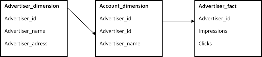
We have two  datasets with 4 cols each with different names. We should create a  dataset with 4 cols 3 from one dataset and one col with the record count of one dataset.

We can use aggregator with a dummy column and get the count from one dataset and do a look up from other dataset and map it to the 3 rd dataset
Something similar to the below design:
Scenario 2:
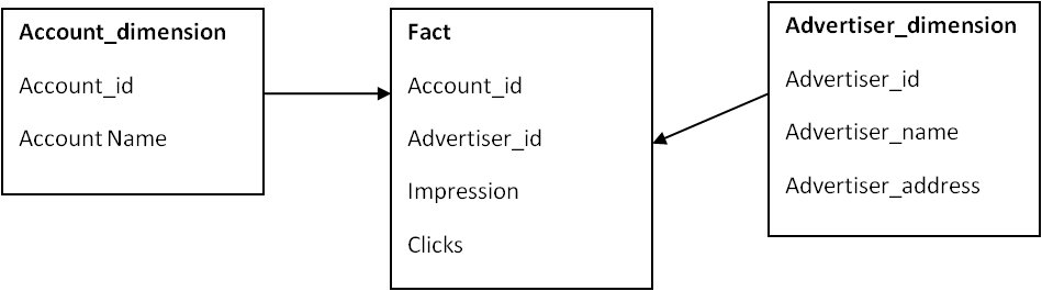
Following is the existing job design. But requirement got changed to: Head and trailer datasets should populate even if detail records is not present in the source file. Below job don't do that job.

Hence changed the above job to this following requirement:
Used row generator with a copy stage. Given default value( zero) for col( count) coming in from row generator. If no detail records it will pick the record count from row generator.


We have a source which is a sequential file with header and footer. How to remove the header and footer while reading this file using sequential file stage of Datastage?
Sol:Type command in putty: sed '1d;$d' file_name>new_file_name (type this in job before job subroutine then use new file in seq stage)

IF I HAVE SOURCE LIKE COL1 A A B AND TARGET LIKE COL1 COL2 A 1 A 2 B1. HOW TO ACHIEVE THIS OUTPUT USING STAGE VARIABLE IN TRANSFORMER STAGE?

If keyChange =1 Then 1 Else stagevaraible+1


Suppose that 4 job control by the sequencer like (job 1, job 2, job 3, job 4 )if job 1 have 10,000 row ,after run the job only 5000 data has been loaded in target table remaining are not loaded and your job going to be aborted then.. How can short out the problem.Suppose job sequencer synchronies or control 4 job but job 1 have problem, in this condition should go director and check it what type of problem showing either data type problem, warning massage, job fail or job aborted, If job fail means data type problem or missing column action .So u should go Run window ->Click-> Tracing->Performance or In your target table ->general -> action-> select this option here two option
(i) On Fail -- commit , Continue
(ii) On Skip -- Commit, Continue.
First u check how many data already load after then select on skip option then continue and what remaining position data not loaded then select On Fail , Continue ...... Again Run the job defiantly u get successful massage
Question: I want to process 3 files in sequentially one by one how can i do that. while processing the files it should fetch files automatically .
Ans:If the metadata for all the files r same then create a job having file name as parameter then use same job in routine and call the job with different file name...or u can create sequencer to use the job..

Parameterize the file name.
Build the job using that parameter
Build job sequencer which will call this job and will accept the parameter for file name.
Write a UNIX shell script which will call the job sequencer three times by passing different file each time.
RE: What Happens if RCP is disable ?

In such case Osh has to perform Import and export every time when the job runs and the processing time job is also increased...
Runtime column propagation (RCP): If RCP is enabled for any job and specifically for those stages whose output connects to the shared container input then meta data will be propagated at run time so there is no need to map it at design time.
If RCP is disabled for the job in such case OSH has to perform Import and export every time when the job runs and the processing time job is also increased.
Then you have to manually enter all the column description in each stage.RCP- Runtime column propagation

Question:
Source:                                                   Target

Eno        Ename                                        Eno           Ename
1                     a,b                                                  1              a
2                     c,d                                                  2              b
3                     e,f                                                  3              c


source has 2 fields like

COMPANY             LOCATION
IBM                  HYD
TCS                  BAN
IBM                  CHE
HCL                  HYD
TCS                  CHE
IBM                  BAN
HCL                  BAN
HCL                  CHE

LIKE THIS.......

THEN THE OUTPUT LOOKS LIKE THIS....

Company loc count

TCS  HYD  3
         BAN
         CHE
IBM  HYD  3
         BAN
         CHE
HCL  HYD  3
         BAN
         CHE
2)input is like this:
no,char
1,a
2,b
3,a
4,b
5,a
6,a
7,b
8,a


But the output is in this form  with row numbering of Duplicate occurence


output:

no,char,Count
"1","a","1"
"6","a","2"
"5","a","3"
"8","a","4"
"3","a","5"
"2","b","1"
"7","b","2"
"4","b","3"
3)Input is like this:
file1
10
20
10
10
20
30

Output is like:
file2               file3(duplicates)
10                  10
20                  10
30                  20

4)Input is like:
file1
10
20
10
10
20
30

Output is like Multiple occurrences in one file and single occurrences in one file:
file2      file3
10         30
10
10
20
20
5)Input is like this:
file1
10
20
10
10
20
30

Output is like:
file2               file3
10                  30
20
6)Input is like this:
file1
1
2
3
4
5
6
7
8
9
10

Output is like:
file2(odd)         file3(even)
1                      2
3                      4
5                      6
7                      8
9                      10
7)How to calculate Sum(sal), Avg(sal), Min(sal), Max(sal) with out using Aggregator stage..

8)How to find out First sal, Last sal in each dept with out using aggregator stage

9)How many ways are there to perform remove duplicates function with out using Remove duplicate stage..

Scenario: 

source has 2 fields like

COMPANY             LOCATION
IBM                  HYD
TCS                  BAN
IBM                  CHE
HCL                  HYD
TCS                  CHE
IBM                  BAN
HCL                  BAN
HCL                  CHE

LIKE THIS.......

THEN THE OUTPUT LOOKS LIKE THIS....

Company loc count

TCS  HYD  3
         BAN
         CHE
IBM  HYD  3
         BAN
         CHE
HCL  HYD  3
         BAN
         CHE

Solution:

Seqfile......>Sort......>Trans......>RemoveDuplicates..........Dataset 

Sort                                             Trans: 
Key=Company                                create stage variable as Company1 
Sort order=Asc                  Company1=If(in.keychange=1) then in.Location Else Company1:',':in.Location 
create keychange=True                          Drag and Drop in derivation 
                                                            Company     ....................Company 
                                                           Company1........................Location 
RemoveDup: 
Key=Company 
Duplicates To Retain=Last 


11)The input is 
Shirt|red|blue|green 
Pant|pink|red|blue 


Output should be, 

Shirt:red 
Shirt:blue 
Shirt:green 
pant:pink 
pant:red 
pant:blue 

Solution:
it is reverse to pivote stage 
use 
     seq------sort------tr----rd-----tr----tg 
in the sort stage use create key change column is true 
in trans create stage variable=if colu=1 then key c.value else key v::colum 
rd stage use duplicates retain last 
tran stage use field function superate columns 

similar Scenario: :
source 
col1 col3 
1 samsung 
1 nokia 
1 ercisson 
2 iphone 
2 motrolla 
3 lava 
3 blackberry 
3 reliance 

Expected Output 
col 1 col2       col3   col4 
1     samsung nokia ercission 
2      iphone   motrolla 
3       lava     blackberry reliance

You can get it  by using    Sort stage --- Transformer stage --- RemoveDuplicates --- Transformer --tgt 


Ok 

First  Read and Load the data  into your  source file( For Example  Sequential File ) 

And  in Sort stage    select key change column = True  ( To Generate  Group ids) 

Go to  Transformer stage   

Create one stage variable. 

You can do this by  right click  in stage variable  go to  properties  and name it as  your wish ( For example temp) 

and  in expression  write as below 

if keychange column =1   then column name   else  temp:',':column name 

This column name is  the one  you want  in the required  column with delimited  commas. 

On remove duplicates stage key is col1 and set option duplicates retain to--> Last. 
in transformer drop col3 and define 3 columns like col2,col3,col4 
in col1 derivation give Field(InputColumn,",",1) and 
in col1 derivation give Field(InputColumn,",",2) and 
in col1 derivation give Field(InputColumn,",",3) 

Scenario: 
12)Consider the following employees data as source? 
employee_id, salary 
------------------- 
10,          1000 
20,          2000 
30,          3000 
40,          5000 

 Create a job to find the sum of salaries of all employees and this sum should repeat for all the rows. 

The output should look like as 

employee_id, salary, salary_sum 
------------------------------- 
10,          1000,   11000 
20,          2000,   11000 
30,          3000,   11000 
40,          5000,   11000

Scenario: 

I have two source tables/files numbered 1 and 2. 
In the the target, there are three output tables/files, numbered 3,4 and 5. 

The scenario is that, 

to the out put 4 -> the records which are common to both 1 and 2 should go. 

to the output 3 -> the records which are only in 1 but not in 2 should go 

to the output 5 -> the records which are only in 2 but not in 1 should go.
sltn:src1----->copy1------>----------------------------------->output_1(only left table) 
                                     Join(inner type)----> ouput_1 
src2----->copy2------>----------------------------------->output_3(only right table)


Consider the following employees data as source? 
employee_id, salary 
------------------- 
10,          1000 
20,          2000 
30,          3000 
40,          5000 

Scenario: 

 Create a job to find the sum of salaries of all employees and this sum should repeat for all the rows. 

The output should look like as 

employee_id, salary, salary_sum 
------------------------------- 
10,          1000,   11000 
20,          2000,   11000 
30,          3000,   11000 
40,          5000,   11000 
sltn:

Take Source --->Transformer(Add new Column on both the output links and assign a value  as 1 )------------------------>                           1) Aggregator  (Do group by  using that new column) 
                                              2)lookup/join( join on that  new column)-------->tgt. 

Scenario: 
sno,sname,mark1,mark2,mark3 
1,rajesh,70,68,79 
2,mamatha,39,45,78 
3,anjali,67,39,78 
4,pavani,89,56,45 
5,indu,56,67,78 

out put is 
sno,snmae,mark1,mark2,mark3,delimetercount 
1,rajesh,70,68,79,4 
2,mamatha,39,45,78,4 
3,anjali,67,39,78,4 
4,pavani,89,56,45,4 
5,indu,56,67,78,4 

seq--->trans--->seq 

create one stage variable as delimiter.. 
and put derivation on stage as DSLink4.sno : "," : DSLink4.sname : "," : DSLink4.mark1 :  "," :DSLink4.mark2 :  "," : DSLink4.mark3 


and do mapping and create one more column count as integer type. 

and put derivation on count column as  Count(delimter, ",") 


scenario: 
       sname         total_vowels_count 
       Allen                          2 
       Scott                          1 
       Ward                         1 
Under Transformer Stage Description: 

total_Vowels_Count=Count(DSLink3.last_name,"a")+Count(DSLink3.last_name,"e")+Count(DSLink3.last_name,"i")+Count(DSLink3.last_name,"o")+Count(DSLink3.last_name,"u").

Scenario: 

1)On daily we r getting some huge files data so all files metadata is same we have to load in to target table how we can load? 
Use File Pattern in sequential file 

2) One column having 10 records at run time we have to send 5th and 6th record to target at run time how we can send? 
Can get through,by using UNIX command in sequential file  filter option

How can we get 18 months date data in transformer stage? 
Use transformer  stage after input seq file  and  try  this  one  as constraint in transformer stage : 

DaysSinceFromDate(CurrentDate(), DSLink3.date_18)<=548 OR DaysSinceFromDate(CurrentDate(), DSLink3.date_18)<=546 

where  date_18  column is the column having that  date  which  needs to be less or equal to 18 months and 548 is  no. of days  for 18 months  and  for leap year it is 546(these  numbers  you need to check). 

What is differences between Force Compile and Compile ?


Diff b/w Compile and Validate?
Compile option only checks for all mandatory requirements like link requirements, stage options and all. But it will not check if the database connections are valid. 
Validate is equivalent to Running a job except for extraction/loading of data. That is, validate option will test database connectivity by making connections to databases. 


How to FInd Out Duplicate Values Using Transformer?


You can capture the duplicate records based on keys using Transformer stage variables.

1. Sort and partition the input data of the transformer on the key(s) which defines the duplicate.
2. Define two stage variables, let's say StgVarPrevKeyCol(data type same as KeyCol) and StgVarCntr as Integer with default value 0
where KeyCol is your input column which defines the duplicate.

Expression for StgVarCntr(1st stg var-- maintain order):

If DSLinknn.KeyCol = StgVarPrevKeyCol Then StgVarCntr + 1 Else 1

Expression for StgVarPrevKeyCol(2nd stg var):

DSLinknn.KeyCol

3. Now in constrain, if you filter rows where StgVarCntr = 1 will give you the unique records and if you filter StgVarCntr > 1 will give you duplicate records.

My source is Like
Sr_no, Name
10,a
10,b
20,c
30,d
30,e
40,f

My target Should Like:

Target 1:(Only unique means which records r only once)
20,c
40,f

Target 2:(Records which r having more than 1 time)
10,a
10,b
30,d
30,e

How to do this in DataStage....

**************

use aggregator and transformer stages

source-->aggregator-->transformat-->target

perform count in aggregator, and take two op links in trasformer, filter data count>1 for one llink and put count=1 for second link.
Scenario: 
in my i/p source i have N no.of records

In output i have 3 targets

i want o/p like 1st rec goes to 1st targt and

2nd rec goes to 2nd target and

3rd rec goes to 3rd target again

4th rec goes to 1st taget ............ like this

do this ""without using partition techniques "" remember it.

*****************
source--->trans---->target
in trans use conditions on constraints
mod(empno,3)=1
mod(empno,3)=2
mod(empno,3)=0
Scenario:
im having i/p as
col A
a_b_c
x_F_I
DE_GH_IF

we hav to mak it as

col1 col 2 col3
a b c
x f i
de gh if


*********************

Transformer
create 3 columns with derivation
col1 Field(colA,'_',1)
col2 Field(colA,'_',2)
col3 Field(colA,'_',3)

**************
Field function divides the column based on the delimeter,
if the data in the col is like A,B,C
then
Field(col,',',1) gives A
Field(col,',',2) gives B
Field(col,',',3) gives C

Scenario:

Scenario:
Scenario:

Friday, October 23, 2015

Compile a Datastage job/multiple jobs through Command Line

Question

How do you compile all jobs in a project via command line?

Answer

Perform the following:
  1. Open a DOS command prompt on the client
  2. Run the following from C:\IBM\InformationServer\Clients\Classic:

    dscc.exe /H hostname /U username /P password project_name /J jobname

    Note: The job name can be * to compile all the jobs in the Project.

Note: you cannot use this command to compile a single job.

Thursday, October 22, 2015

Datastage All Stages

Datastage parallel stages groups

DataStage and QualityStage stages are grouped into the following logical sections: 
  • General objects
  • Data Quality Stages
  • Database connectors
  • Development and Debug stages
  • File stages
  • Processing stages
  • Real Time stages
  • Restructure Stages
  • Sequence activities
Please refer to the list below for a description of the stages used in DataStage and QualityStage. 
We classified all stages in order of importancy and frequency of use in real-life deployments (and also on certification exams). Also, the most widely used stages are marked bold or there is a link to a subpage available with a detailed description with examples. 

DataStage and QualityStage parallel stages and activities

General stages

General elements


  • Link indicates a flow of the data. There are three main types of links in Datastage: stream, reference and lookup.

    • Container (can be private or shared) - the main outcome of having containers is to simplify visually a complex datastage job design and keep the design easy to understand.
    • Annotation is used for adding floating datastage job notes and descriptions on a job canvas. Annotations provide a great way to document the ETL process and help understand what a given job does.
    • Description Annotation shows the contents of a job description field. One description annotation is allowed in a datastage job.


    Debug and development stages

    Debug and development stages

    • Row generator produces a set of test data which fits the specified metadata (can be random or cycled through a specified list of values). Useful for testing and development. Click here for more..
    • Column generator adds one or more column to the incoming flow and generates test data for this column.
    • Peek stage prints record column values to the job log which can be viewed in Director. It can have a single input link and multiple output links.Click here for more..
    • Sample stage samples an input data set. Operates in two modes: percent mode and period mode.
    • Head selects the first N rows from each partition of an input data set and copies them to an output data set.
    • Tail is similiar to the Head stage. It select the last N rows from each partition.
    • Write Range Map writes a data set in a form usable by the range partitioning method.
    Processing stages

    Processing stages

    • Aggregator joins data vertically by grouping incoming data stream and calculating summaries (sum, count, min, max, variance, etc.) for each group. The data can be grouped using two methods: hash table or pre-sort. Click herefor more..
    • Copy - copies input data (a single stream) to one or more output data flows
    • FTP stage uses FTP protocol to transfer data to a remote machine
    • Filter filters out records that do not meet specified requirements.Click here for more..
    • Funnel combines mulitple streams into one. Click here for more..
    • Join combines two or more inputs according to values of a key column(s). Similiar concept to relational DBMS SQL join (ability to perform inner, left, right and full outer joins). Can have 1 left and multiple right inputs (all need to be sorted) and produces single output stream (no reject link). Click here for more..
    • Lookup combines two or more inputs according to values of a key column(s). Lookup stage can have 1 source and multiple lookup tables. Records don't need to be sorted and produces single output stream and a reject link. Clickhere for more..
    • Merge combines one master input with multiple update inputs according to values of a key column(s). All inputs need to be sorted and unmatched secondary entries can be captured in multiple reject links. Click here for more..
    • Modify stage alters the record schema of its input dataset. Useful for renaming columns, non-default data type conversions and null handling
    • Remove duplicates stage needs a single sorted data set as input. It removes all duplicate records according to a specification and writes to a single output
    • Slowly Changing Dimension automates the process of updating dimension tables, where the data changes in time. It supports SCD type 1 and SCD type 2.Click here for more..
    • Sort sorts input columns.Click here for more..
    • Transformer stage handles extracted data, performs data validation, conversions and lookups.Click here for more..
    • Change Capture - captures before and after state of two input data sets and outputs a single data set whose records represent the changes made.
    • Change Apply - applies the change operations to a before data set to compute an after data set. It gets data from a Change Capture stage
    • Difference stage performs a record-by-record comparison of two input data sets and outputs a single data set whose records represent the difference between them. Similiar to Change Capture stage.
    • Checksum - generates checksum from the specified columns in a row and adds it to the stream. Used to determine if there are differencies between records.
    • Compare performs a column-by-column comparison of records in two presorted input data sets. It can have two input links and one output link.
    • Encode encodes data with an encoding command, such as gzip.
    • Decode decodes a data set previously encoded with the Encode Stage.
    • External Filter permits speicifying an operating system command that acts as a filter on the processed data
    • Generic stage allows users to call an OSH operator from within DataStage stage with options as required.
    • Pivot Enterprise is used for horizontal pivoting. It maps multiple columns in an input row to a single column in multiple output rows. Pivoting data results in obtaining a dataset with fewer number of columns but more rows.
    • Surrogate Key Generator generates surrogate key for a column and manages the key source.
    • Switch stage assigns each input row to an output link based on the value of a selector field. Provides a similiar concept to the switch statement in most programming languages.
    • Compress - packs a data set using a GZIP utility (or compress command on LINUX/UNIX)
    • Expand extracts a previously compressed data set back into raw binary data.
    Database stages

    File stage types

    • Sequential file is used to read data from or write data to one or more flat (sequential) files.Click here for more..
    • Data Set stage allows users to read data from or write data to a dataset. Datasets are operating system files, each of which has a control file (.ds extension by default) and one or more data files (unreadable by other applications). Click here for more info
    • File Set stage allows users to read data from or write data to a fileset. Filesets are operating system files, each of which has a control file (.fs extension) and data files. Unlike datasets, filesets preserve formatting and are readable by other applications.
    • Complex flat file allows reading from complex file structures on a mainframe machine, such as MVS data sets, header and trailer structured files, files that contain multiple record types, QSAM and VSAM files.Click here for more info.
    • External Source - permits reading data that is output from multiple source programs.
    • External Target - permits writing data to one or more programs.
    • Lookup File Set is similiar to FileSet stage. It is a partitioned hashed file which can be used for lookups.
    Database stages

    Database stages


    • Oracle Enterprise allows reading data from and writing data to an Oracle database (database version from 9.x to 10g are supported).
    • ODBC Enterprise permits reading data from and writing data to a database defined as an ODBC source. In most cases it is used for processing data from or to Microsoft Access databases and Microsoft Excel spreadsheets.
    • DB2/UDB Enterprise permits reading data from and writing data to a DB2 database.
    • Teradata permits reading data from and writing data to a Teradata data warehouse. Three Teradata stages are available: Teradata connector, Teradata Enterprise and Teradata Multiload
    • SQLServer Enterprise permits reading data from and writing data to Microsoft SQLl Server 2005 amd 2008 database.
    • Sybase permits reading data from and writing data to Sybase databases.
    • Stored procedure stage supports Oracle, DB2, Sybase, Teradata and Microsoft SQL Server. The Stored Procedure stage can be used as a source (returns a rowset), as a target (pass a row to a stored procedure to write) or a transform (to invoke procedure processing within the database).
    • MS OLEDB helps retrieve information from any type of information repository, such as a relational source, an ISAM file, a personal database, or a spreadsheet.
    • Dynamic Relational Stage (Dynamic DBMS, DRS stage) is used for reading from or writing to a number of different supported relational DB engines using native interfaces, such as Oracle, Microsoft SQL Server, DB2, Informix and Sybase.
    • Informix (CLI or Load)
    • DB2 UDB (API or Load)
    • Classic federation
    • RedBrick Load
    • Netezza Enterpise
    • iWay Enterprise
    Real time

    Real Time stages

    • XML Input stage makes it possible to transform hierarchical XML data to flat relational data sets
    • XML Output writes tabular data (relational tables, sequential files or any datastage data streams) to XML structures
    • XML Transformer converts XML documents using an XSLT stylesheet
    • Websphere MQ stages provide a collection of connectivity options to access IBM WebSphere MQ enterprise messaging systems. There are two MQ stage types available in DataStage and QualityStage: WebSphere MQ connector and WebSphere MQ plug-in stage.
    • Web services client
    • Web services transformer
    • Java client stage can be used as a source stage, as a target and as a lookup. The java package consists of three public classes: com.ascentialsoftware.jds.Column, com.ascentialsoftware.jds.Row, com.ascentialsoftware.jds.Stage
    • Java transformer stage supports three links: input, output and reject.
    • WISD Input - Information Services Input stage
    • WISD Output - Information Services Output stage
    Real time

    Restructure stages

    • Column export stage exports data from a number of columns of different data types into a single column of data type ustring, string, or binary. It can have one input link, one output link and a rejects link. Click here for more..
    • Column import complementary to the Column Export stage. Typically used to divide data arriving in a single column into multiple columns.
    • Combine records stage combines rows which have identical keys, into vectors of subrecords.
    • Make subrecord combines specified input vectors into a vector of subrecords whose columns have the same names and data types as the original vectors.
    • Make vector joins specified input columns into a vector of columns
    • Promote subrecord - promotes input subrecord columns to top-level columns
    • Split subrecord - separates an input subrecord field into a set of top-level vector columns
    • Split vector promotes the elements of a fixed-length vector to a set of top-level columns
    Data quality QualityStage

    Data quality QualityStage stages

    • Investigate stage analyzes data content of specified columns of each record from the source file. Provides character and word investigation methods.
    • Match frequency stage takes input from a file, database or processing stages and generates a frequence distribution report.
    • MNS - multinational address standarization.
    • QualityStage Legacy
    • Reference Match
    • Standarize
    • Survive
    • Unduplicate Match
    • WAVES - worldwide address verification and enhancement system.


    Sequence activities

    Sequence activity stage types

    • Job Activity specifies a Datastage server or parallel job to execute.
    • Notification Activity - used for sending emails to user defined recipients from within Datastage
    • Sequencer used for synchronization of a control flow of multiple activities in a job sequence.
    • Terminator Activity permits shutting down the whole sequence once a certain situation occurs.
    • Wait for file Activity - waits for a specific file to appear or disappear and launches the processing.
    • EndLoop Activity
    • Exception Handler
    • Execute Command
    • Nested Condition
    • Routine Activity
    • StartLoop Activity
    • UserVariables Activity    

    python

      import datetime import pandas as pd import cx_Oracle con = cx_Oracle.connect( 'SYSTEM/oracle123@localhost:1521/xe' ) c = con.c...